We’ll use Rock, Paper, Scissors dataset created by Laurence Moroney (lmoroney@gmail.com / laurencemoroney.com ) and can be found in his site: Rock Paper Scissors Dataset .
The dataset is licensed as Creative Commons (CC BY 2.0). No changes were made to the dataset.
Code
from IPython.display import display, HTML"<style>.container { width:80% !important; }</style>" ))import numpy as npimport torchimport torch.optim as optimimport torch.nn as nnfrom shared.step_by_step import StepByStepimport platformfrom PIL import Imageimport datetimeimport matplotlib.pyplot as pltfrom matplotlib import cmfrom torch.utils.data import DataLoader, Dataset, TensorDataset, random_split, WeightedRandomSampler, SubsetRandomSamplerfrom torchvision.transforms import Compose, ToTensor, Normalize, ToPILImage, RandomHorizontalFlip, Resize, CenterCropfrom tqdm.autonotebook import tqdmfrom torch.optim.lr_scheduler import StepLR, ReduceLROnPlateau, MultiStepLR, CyclicLR, LambdaLRfrom torchvision.datasets import ImageFolderfrom shared.rps import download_rps'fivethirtyeight' )
Code
def show_image(im, cmap= None ):= plt.figure(figsize= (3 ,3 ))= cmap)False )
Data
Temporary dataset
We need to calculate normalization parameters (mean and std) for all training images first. This is important step as we will use these normalization parameters not only for training images but for all the validation, and any future, predictions. Since we need to only calculate normalization parameters, we can also scale images to smaller size, just so the calculation is faster.
= Compose([Resize(28 ),= ImageFolder(root= 'rps' , transform= composer)= DataLoader(temp_dataset, batch_size= 32 )= StepByStep.make_normalizer(temp_loader)
Real dataset
= Compose([Resize(28 ), ToTensor(), normalizer])= ImageFolder(root= 'rps' , transform= composer)= ImageFolder(root= 'rps-test-set' , transform= composer)= DataLoader(train_dataset, batch_size= 16 , shuffle= True )= DataLoader(val_dataset, batch_size= 16 )
= next (iter (train_loader))
<torch.utils.data.dataloader.DataLoader>
tensor([2, 0, 2, 0, 0, 2, 1, 0, 1, 2, 0, 2, 1, 2, 0, 1])
Deep model
We’ll use CrossEntropyLoss (and not add LogSoftmax layer):
class CNN2(nn.Module):def __init__ (self , n_filters, p= 0.3 ):super (CNN2, self ).__init__ ()self .n_filters = n_filtersself .p = p# conv1 takes (3,28,28) and outputs (n_filters,26,26) self .conv1 = nn.Conv2d(= 3 , = n_filters, = 3 # conv2 takes (n_filters,13,13) and outputs (n_filters,11,11) self .conv2 = nn.Conv2d(= n_filters, = n_filters, = 3 self .fc1 = nn.Linear(n_filters* 5 * 5 , 50 )self .fc2 = nn.Linear(50 ,3 )self .drop = nn.Dropout(p)def featurizer(self , x):= self .conv1(x)= nn.ReLU()(x)= nn.MaxPool2d(kernel_size= 2 )(x) # (n_filters,13,13) = self .conv2(x) # n_filters,11, 11 = nn.ReLU()(x)= nn.MaxPool2d(kernel_size= 2 )(x) # (n_filters,5,5) = nn.Flatten()(x)return xdef classifier(self , x):if self .p > 0 := self .drop(x)= self .fc1(x)= nn.ReLU()(x)if self .p > 0 := self .drop(x)= self .fc2(x)= nn.Flatten()(x)return xdef forward(self , x):= self .featurizer(x)= self .classifier(x)return x
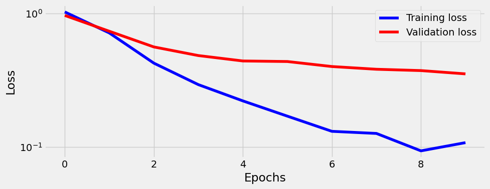
= CNN2(5 , 0.3 )= optim.Adam(model_cnn.parameters(), lr= 3e-4 )= nn.CrossEntropyLoss()
= StepByStep(model_cnn, optimizer_cnn, multi_loss_fn)
Code
print ('Correct categories:' )print (sbs.loader_apply(sbs.val_loader, sbs.correct))
Correct categories:
tensor([[ 90, 124],
        [ 94, 124],
        [104, 124]])
Code
print (f'Accuracy: { sbs. accuracy} %' )
100%|█████████████████████████████████████████████████████████████████████████████████████████████████████████████████████████████████████████████████████████████████████████████████████████████████| 30/30 [05:03<00:00, 10.12s/it]
Code
print ('Correct categories:' )print (sbs.loader_apply(sbs.val_loader, sbs.correct))
Correct categories:
tensor([[107, 124],
        [103, 124],
        [105, 124]])
Code
print (f'Accuracy: { sbs. accuracy} %' )
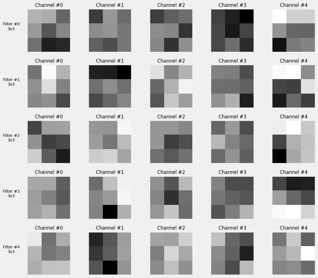
Visualize filters
= sbs.visualize_filters('conv2' , cmap= 'gray' )
Not too informative.
Learning Rate Finder
There is an off-the-shelf LRFinder:
#!pip install --quiet torch-lr-finder
from torch_lr_finder import LRFinder
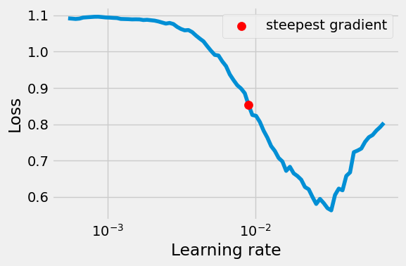
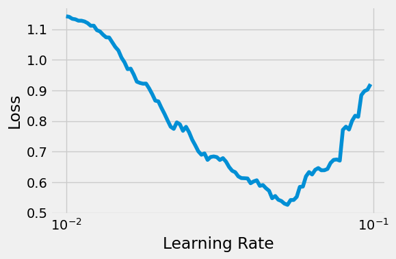
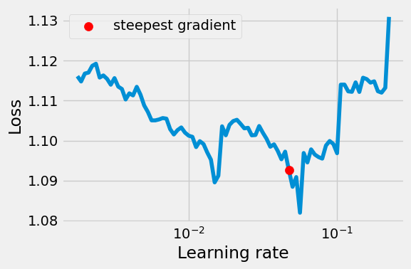
= plt.subplots(1 , 1 , figsize= (6 , 4 ))11 )= CNN2(5 , 0.3 )= nn.CrossEntropyLoss(reduction= 'mean' )= optim.Adam(model_cnn.parameters(), lr= 3e-4 )= 'cuda' if torch.cuda.is_available() else 'cpu' = LRFinder(model_cnn, optimizer, multi_loss_fn, device= device)= 1e-1 , num_iter= 100 )= ax, log_lr= True )
Learning rate search finished. See the graph with {finder_name}.plot()
LR suggestion: steepest gradient
Suggested LR: 9.02E-03
We can replicate the above by using scheduler module torch.optim.lr_scheduler for example LambdaLR (there are other schedulers: StepLR, ReduceLROnPlateau, MultiStepLR, CyclicLR). These work by steping through iterations of learning rates, using step method (similar to optimizer step).
We first define a function that can make linear or exponential scalling factors between start_lr and end_lr:
def make_lr_fn(start_lr, end_lr, num_iter, step_mode= 'exp' ):if step_mode == 'linear' := (end_lr / start_lr - 1 ) / num_iterdef lr_fn(iteration):return 1 + iteration * factorelse := (np.log(end_lr) - np.log(start_lr)) / num_iter def lr_fn(iteration):return np.exp(factor)** iteration return lr_fn
If we now make optimizer and scheduler, we can step through and see that learning late changes with each step:
= optim.Adam(model_cnn.parameters(), lr= 0.01 )= LambdaLR(optimizer_cnn, lr_lambda= make_lr_fn(0.01 , 0.1 , 10 ))
for _ in range (3 ):print (scheduler.get_last_lr())
[0.01]
[0.012589254117941673]
[0.015848931924611138]
We can make a lr_range_test method that is using this scheduler, and use it to plot the loss for different learning rates:
13 )= CNN2(5 )= nn.CrossEntropyLoss()= optim.Adam(model_cnn.parameters(), lr= 0.01 )= StepByStep(model_cnn, optimizer_cnn, multi_loss_fn)= sbs.lr_range_test(train_loader, end_lr= 1e-1 , num_iter= 100 )
And this is basically identical to the off-the-shelf one.
Repeated lr_range_test gives slightly differnt graph but doesn’t affect the model and optimizer states.
= sbs.lr_range_test(train_loader, end_lr= 1e-1 , num_iter= 100 )
Adam - adaptive gradients
Adam is optimizer that instead of gradients (used in SGD) calculates adaptive_gradients , taking bias-corrected exponentially-weighted moving average (EWMA) of gradients and gradients squared. This makes convergence to the minimum loss faster then in a regular SGD.
\[
\large \text{adapted-gradient}_t = \frac{\text{Bias Corrected EWMA}_t(\beta_1, \text{gradients})}{\sqrt{\text{Bias Corrected EWMA}_t(\beta_2, \text{gradients}^2)}+\epsilon}
\]
\[
\Large
\begin{aligned}
\ \text{SGD}: &\text{param}_t = \text{param}_{t-1} - \eta\ \text{gradient}_t
\\
\text{Adam}: &\text{param}_t = \text{param}_{t-1} - \eta\ \text{adapted gradient}_t
\end{aligned}
\]
Basic Adam definition from PyTorch: optim.Adam(params, lr=0.001, betas=(0.9, 0.999), eps=1e-08).
SGD - with momentum
SGD also has variations that are used in practice (especially after being combined with scheduler), these variations are Momentum and Nestorov:
\[
\Large
\begin{aligned}
\ \text{SGD}: &\text{param}_t = \text{param}_{t-1} &-& \eta\ \text{grad}_t
\\
\text{SGD with Momentum}: &\text{param}_t = \text{param}_{t-1} &&&-&& \eta\ \text{mo}_t
\\
\text{SGD with Nesterov}: &\text{param}_t = \text{param}_{t-1} &-& \eta\ \text{grad}_t &-&\beta &\eta\ \text{mo}_t
\end{aligned}
\]
They are invoked using parameters:
optim.SGD(params, lr=<required parameter>, momentum=0, dampening=0, weight_decay=0, nesterov=False)
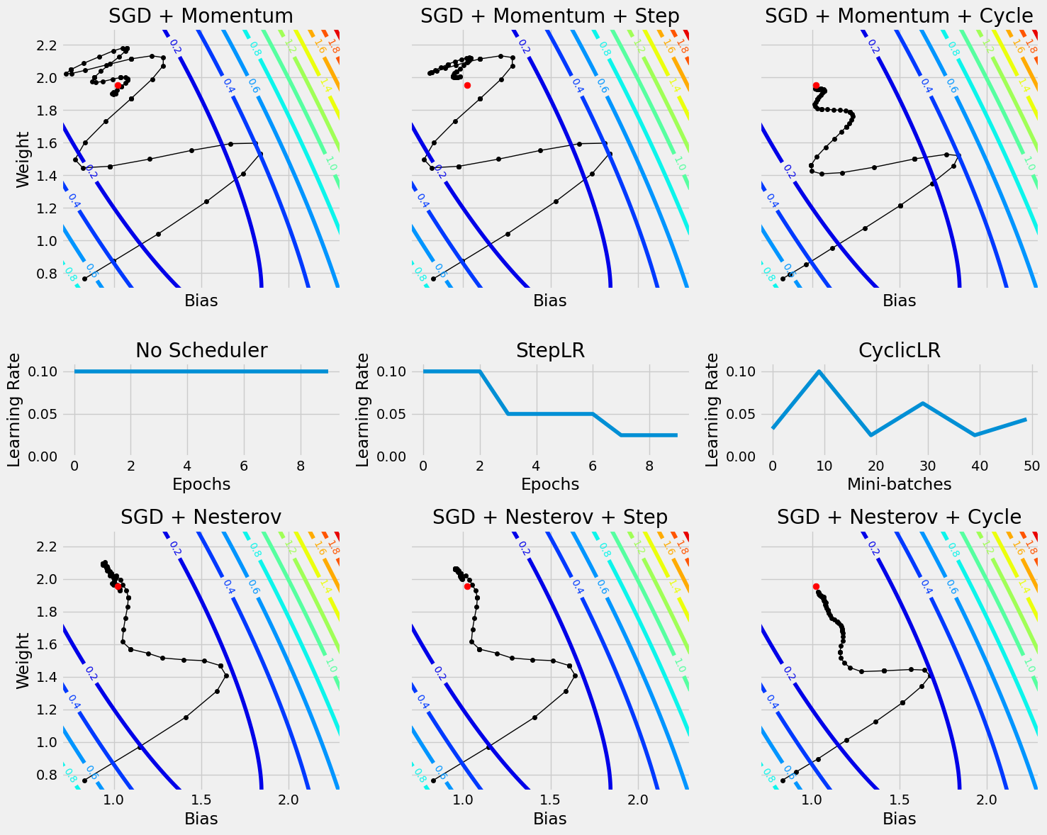
Schedulers
We can combine any optimizer with Schedulers. The general idea behind using a scheduler is to allow the optimizer to alternate between exploring the loss surface (high learning rate phase) and targeting a minimum (low learning rate phase).
Let’s increase the dropout rate for fun:
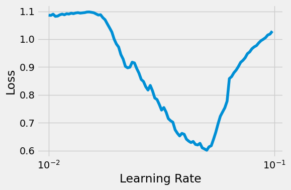
= plt.subplots(1 , 1 , figsize= (6 , 4 ))13 )= CNN2(n_filters= 5 , p= 0.5 )= nn.CrossEntropyLoss(reduction= 'mean' )= optim.SGD(model_cnn3.parameters(), lr= 1e-3 , momentum= 0.9 , nesterov= True )= 'cuda' if torch.cuda.is_available() else 'cpu' = LRFinder(model_cnn3, optimizer_cnn3, multi_loss_fn, device= device)= 3e-1 , num_iter= 100 )= ax, log_lr= True )
Learning rate search finished. See the graph with {finder_name}.plot()
LR suggestion: steepest gradient
Suggested LR: 4.75E-02
the LRFinder curve doesn’t look as pretty as before, but does the job.
Let’s go with the suggestion of 4.75e-2:
So without the Scheduler:
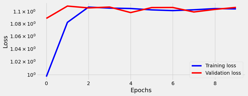
13 )= CNN2(n_filters= 5 , p= 0.5 )= nn.CrossEntropyLoss(reduction= 'mean' )= optim.SGD(model_cnn3.parameters(), lr= 0.0475 , momentum= 0.9 , nesterov= True )= StepByStep(model_cnn3, optimizer_cnn3, multi_loss_fn)10 )
100%|█████████████████████████████████████████████████████████████████████████████████████████████████████████████████████████████████████████████████████████████████████████████████████████████████| 10/10 [01:38<00:00, 9.88s/it]
= sbs_cnn3.plot_losses()print (StepByStep.loader_apply(train_loader, sbs_cnn3.correct).sum (axis= 0 ), sum (axis= 0 ))
tensor([ 840, 2520]) tensor([124, 372])
And this is quite bad loss curve, since lr is quite high.
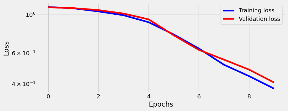
With the Scheduler however:
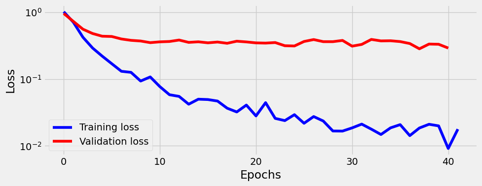
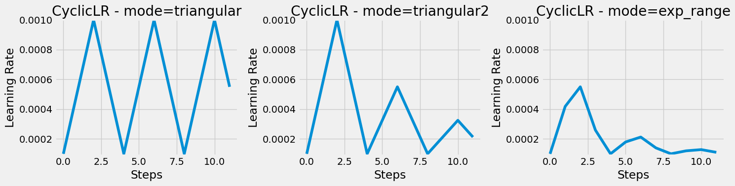
13 )= CNN2(n_filters= 5 , p= 0.5 )= nn.CrossEntropyLoss(reduction= 'mean' )= optim.SGD(model_cnn3.parameters(), lr= 0.0475 , momentum= 0.9 , nesterov= True )= StepByStep(model_cnn3, optimizer_cnn3, multi_loss_fn)= CyclicLR(optimizer_cnn3, base_lr= 1e-3 , max_lr= 5e-2 , step_size_up= len (train_loader), mode= 'triangular2' )10 )
100%|█████████████████████████████████████████████████████████████████████████████████████████████████████████████████████████████████████████████████████████████████████████████████████████████████| 10/10 [01:36<00:00, 9.67s/it]
= sbs_cnn3.plot_losses()print (StepByStep.loader_apply(train_loader, sbs_cnn3.correct).sum (axis= 0 ), sum (axis= 0 ))
tensor([2483, 2520]) tensor([304, 372])
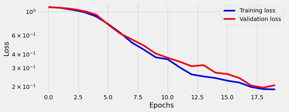
100%|█████████████████████████████████████████████████████████████████████████████████████████████████████████████████████████████████████████████████████████████████████████████████████████████████| 10/10 [01:37<00:00, 9.74s/it]
= sbs_cnn3.plot_losses()print (StepByStep.loader_apply(train_loader, sbs_cnn3.correct).sum (axis= 0 ), sum (axis= 0 ))
tensor([2505, 2520]) tensor([336, 372])
90.3% accuracy is comparable with Adam optimizer used initially (even though Dropout rate was 0.3).
Extra training doesn’t help btw, one could play for example with n_filters, or different model.