Statistics

import matplotlib.pyplot as plt

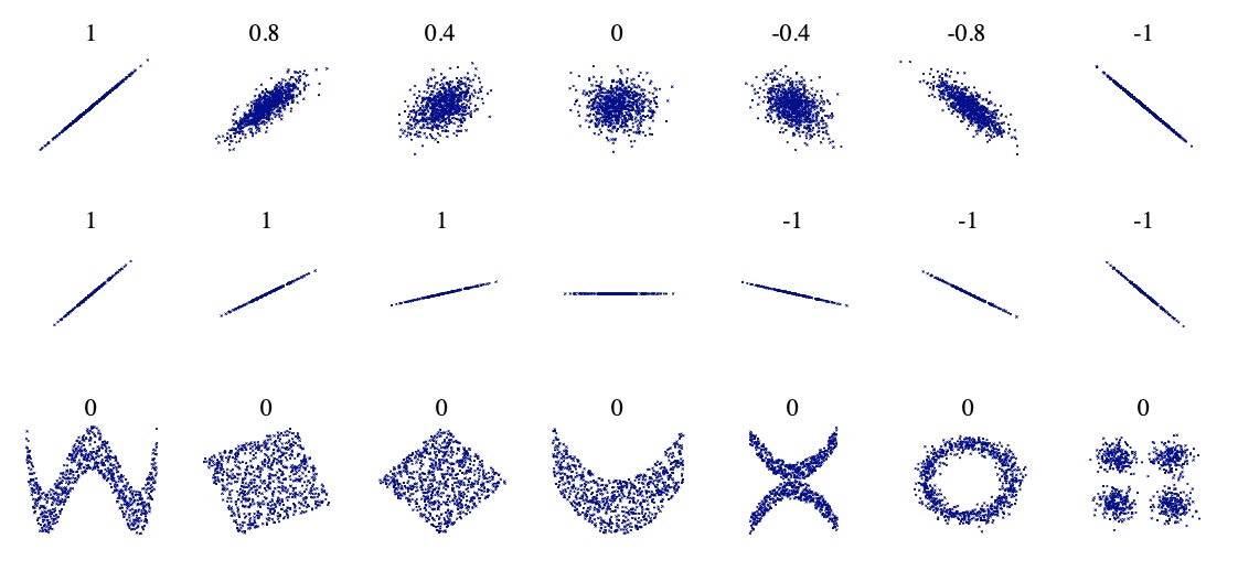
Correlation

Paerson coefficient between columns is a way of measuring a linear correlation. It is a number between –1 and 1 that measures the strength and direction of the relationship between two variables: \(\rho_{X,Y} = \frac{cov(X,Y)}{\sigma_X \sigma_Y} = \frac{(X,Y)}{\sigma_X \sigma_Y}\)

Label Encoder

LabelEncoder can be used to normalize labels.

>>> from sklearn import preprocessing
>>> le = preprocessing.LabelEncoder()
>>> le.fit([1, 2, 2, 6])
LabelEncoder()
>>> le.classes_
array([1, 2, 6])
>>> le.transform([1, 1, 2, 6])
array([0, 0, 1, 2]...)
>>> le.inverse_transform([0, 0, 1, 2])
array([1, 1, 2, 6])

Convert type

df[column].apply(str) df[column].apply(float)

Describe

import pandas as pd
import numpy as np
df = pd.DataFrame(np.random.randn(10, 5), columns=['a', 'b', 'c', 'd', 'e'])
df.describe()

	a	b	c	d	e
count	10.000000	10.000000	10.000000	10.000000	10.000000
mean	0.426285	0.585122	-0.176158	0.060639	-0.362984
std	1.057365	1.221160	1.015207	1.199665	1.178528
min	-0.995421	-0.859328	-1.637495	-1.511699	-1.519060
25%	-0.217827	-0.653228	-0.858613	-0.572152	-0.937348
50%	0.277748	0.764875	-0.043677	-0.241223	-0.733161
75%	0.697302	1.373044	0.206896	0.325958	-0.234405
max	2.446587	2.387042	1.694069	2.220635	2.704051

Missing values visualization

df.iloc[1,2] = np.nan
df.iloc[3,4] = np.nan

import missingno as msno
msno.matrix(df)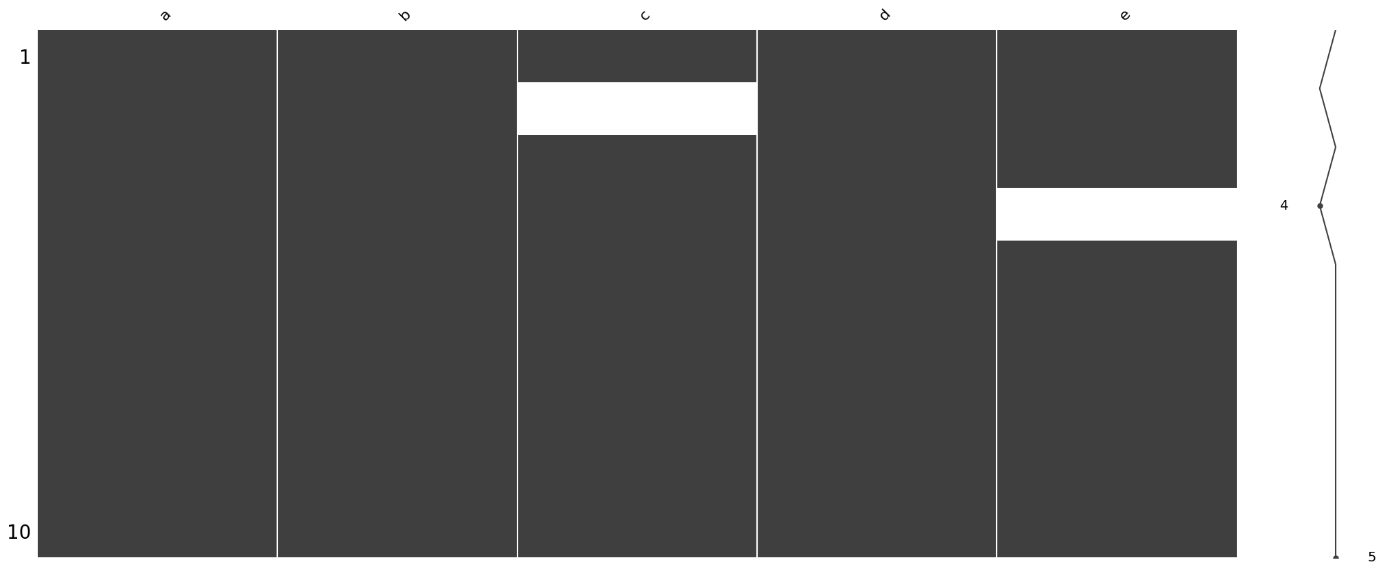

df['c'].fillna(0, inplace=True)

msno.matrix(df)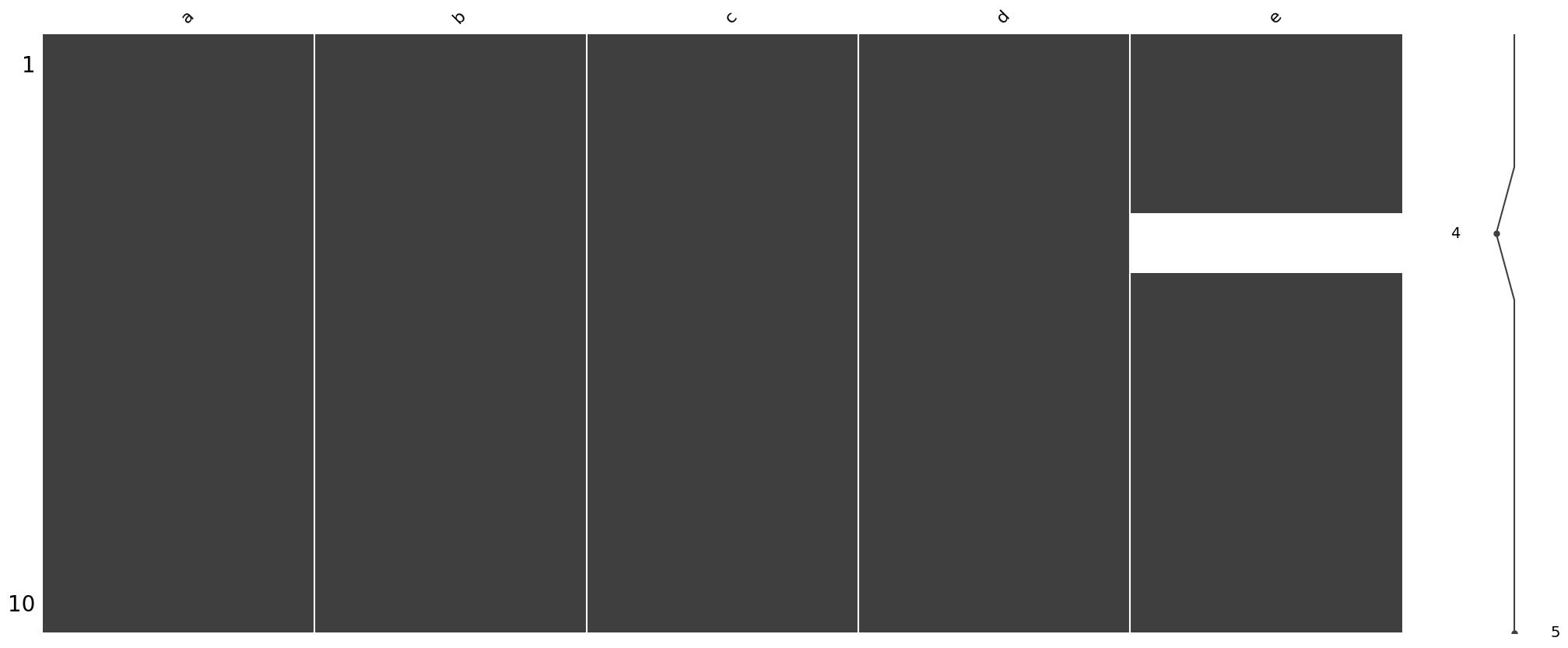

Counter

df.dtypes

a    float64
b    float64
c    float64
d    float64
e    float64
dtype: object

df.a = df.a.apply(str)

df.dtypes

a     object
b    float64
c    float64
d    float64
e    float64
dtype: object

from collections import Counter
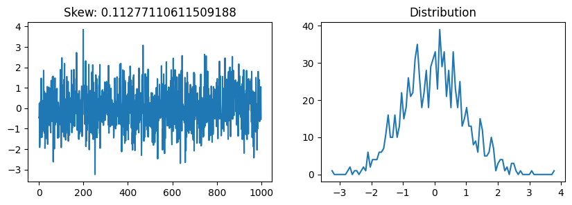
Counter(df.dtypes)

Counter({dtype('O'): 1, dtype('float64'): 4})

Skew

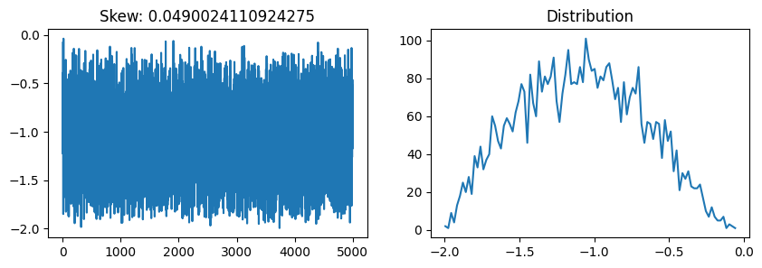
from scipy.stats import skew

def plot_skew(array):
    fig, axs = plt.subplots(1,2, figsize=(10,3))
    axs[0].plot(array)
    values, ranges = np.histogram(array, 100)
    axs[1].plot(ranges[:-1], values)
    axs[0].set_title(f'Skew: {skew(array)}')
    axs[1].set_title('Distribution')
    plt.show()

np.random.seed(42)
plot_skew(np.random.randn(10))
plot_skew(np.random.randn(1000))
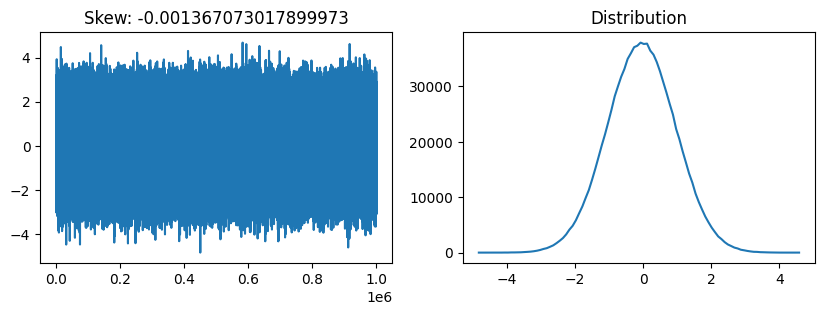
plot_skew(np.random.randn(1000000))
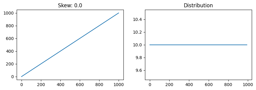
plot_skew(np.arange(1000))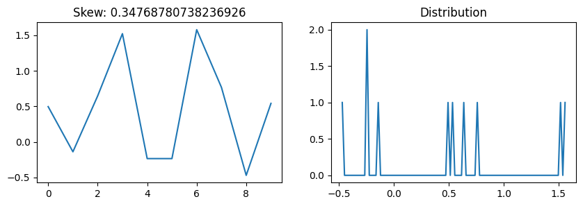

Box-Cox transformation

from scipy.special import boxcox1p
from scipy.special import boxcox

Box-Cox transformation is a way to transform non-normal dependent variables into a normal shape.

a = np.random.beta(1, 3, 5000)

plot_skew(a)
plot_skew(boxcox(a, 0.5))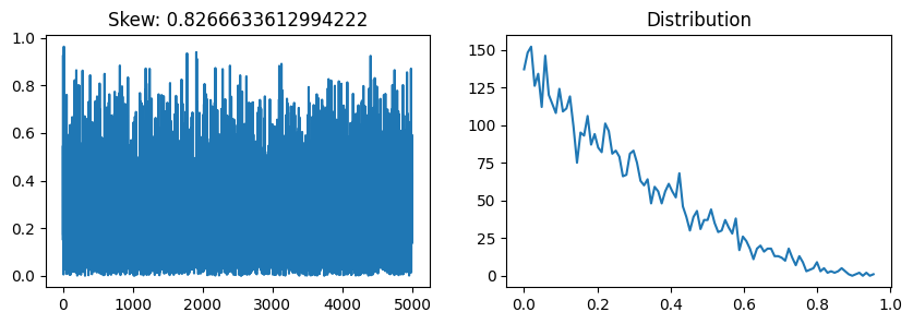

One-hot encoding

s = pd.Series(list('abca'))
s

0    a
1    b
2    c
3    a
dtype: object

pd.get_dummies(s)

	a	b	c
0	1	0	0
1	0	1	0
2	0	0	1
3	1	0	0

Exponential

Calculate exp(x) - 1 for all elements in the array: np.expm1