import numpy as npnp.random.seed(42)a = np.random.randn(1,10)print(a)print(a.max())print(a.dtype)a = a.astype(np.uint8)print(a)print(a.max())print(a.dtype)print(a.shape)a = a.squeeze()print(a.shape)
To scale tensor from 0, 255, convert to uint8
b = (np.array(mask_tensor) / np.array(mask_tensor).max() *255).astype(np.uint8).squeeze()b.max()
b = (np.array(mask_tensor) / np.array(mask_tensor).max()).astype(np.float32).squeeze()b.max()
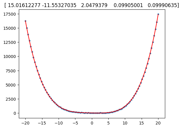
Polynomial fitting
import numpy as npimport matplotlib.pyplot as pltfrom numpy.polynomial import polynomial as PM =100;N =4;x = np.linspace(-20, 20, M)X = np.fliplr(np.vander(x , N +1))# for i in range(N+1):# X[:,i] = x**inoise =20* np.random.randn(M)beta = [18, -12, 2, 0.1, 0.1];y = np.dot(X, beta) + noisebeta_r = np.linalg.solve(X.T.dot(X), X.T.dot(y))y_r = np.dot(X, beta_r)plt.plot(x, y,'.')plt.plot(x, y_r, 'r')plt.title(str(beta_r))plt.show()def plot_something(p): fig, ax = plt.subplots() ax.plot(p, 'o') ax.set_title('Random') plt.show()beta_r, stats = P.polyfit(x, y, 4, full=True)y_r = np.dot(X, beta_r)plt.plot(x, y,'.')plt.plot(x, y_r, 'r')plt.title(str(beta_r))plt.show()help(P.polyfit)
Help on function polyfit in module numpy.polynomial.polynomial:

polyfit(x, y, deg, rcond=None, full=False, w=None)
    Least-squares fit of a polynomial to data.

    Return the coefficients of a polynomial of degree `deg` that is the
    least squares fit to the data values `y` given at points `x`. If `y` is
    1-D the returned coefficients will also be 1-D. If `y` is 2-D multiple
    fits are done, one for each column of `y`, and the resulting
    coefficients are stored in the corresponding columns of a 2-D return.
    The fitted polynomial(s) are in the form

    .. math::  p(x) = c_0 + c_1 * x + ... + c_n * x^n,

    where `n` is `deg`.

    Parameters
    ----------
    x : array_like, shape (`M`,)
        x-coordinates of the `M` sample (data) points ``(x[i], y[i])``.
    y : array_like, shape (`M`,) or (`M`, `K`)
        y-coordinates of the sample points.  Several sets of sample points
        sharing the same x-coordinates can be (independently) fit with one
        call to `polyfit` by passing in for `y` a 2-D array that contains
        one data set per column.
    deg : int or 1-D array_like
        Degree(s) of the fitting polynomials. If `deg` is a single integer
        all terms up to and including the `deg`'th term are included in the
        fit. For NumPy versions >= 1.11.0 a list of integers specifying the
        degrees of the terms to include may be used instead.
    rcond : float, optional
        Relative condition number of the fit.  Singular values smaller
        than `rcond`, relative to the largest singular value, will be
        ignored.  The default value is ``len(x)*eps``, where `eps` is the
        relative precision of the platform's float type, about 2e-16 in
        most cases.
    full : bool, optional
        Switch determining the nature of the return value.  When ``False``
        (the default) just the coefficients are returned; when ``True``,
        diagnostic information from the singular value decomposition (used
        to solve the fit's matrix equation) is also returned.
    w : array_like, shape (`M`,), optional
        Weights. If not None, the weight ``w[i]`` applies to the unsquared
        residual ``y[i] - y_hat[i]`` at ``x[i]``. Ideally the weights are
        chosen so that the errors of the products ``w[i]*y[i]`` all have the
        same variance.  When using inverse-variance weighting, use
        ``w[i] = 1/sigma(y[i])``.  The default value is None.

        .. versionadded:: 1.5.0

    Returns
    -------
    coef : ndarray, shape (`deg` + 1,) or (`deg` + 1, `K`)
        Polynomial coefficients ordered from low to high.  If `y` was 2-D,
        the coefficients in column `k` of `coef` represent the polynomial
        fit to the data in `y`'s `k`-th column.

    [residuals, rank, singular_values, rcond] : list
        These values are only returned if ``full == True``

        - residuals -- sum of squared residuals of the least squares fit
        - rank -- the numerical rank of the scaled Vandermonde matrix
        - singular_values -- singular values of the scaled Vandermonde matrix
        - rcond -- value of `rcond`.

        For more details, see `numpy.linalg.lstsq`.

    Raises
    ------
    RankWarning
        Raised if the matrix in the least-squares fit is rank deficient.
        The warning is only raised if ``full == False``.  The warnings can
        be turned off by:

        >>> import warnings
        >>> warnings.simplefilter('ignore', np.RankWarning)

    See Also
    --------
    numpy.polynomial.chebyshev.chebfit
    numpy.polynomial.legendre.legfit
    numpy.polynomial.laguerre.lagfit
    numpy.polynomial.hermite.hermfit
    numpy.polynomial.hermite_e.hermefit
    polyval : Evaluates a polynomial.
    polyvander : Vandermonde matrix for powers.
    numpy.linalg.lstsq : Computes a least-squares fit from the matrix.
    scipy.interpolate.UnivariateSpline : Computes spline fits.

    Notes
    -----
    The solution is the coefficients of the polynomial `p` that minimizes
    the sum of the weighted squared errors

    .. math:: E = \sum_j w_j^2 * |y_j - p(x_j)|^2,

    where the :math:`w_j` are the weights. This problem is solved by
    setting up the (typically) over-determined matrix equation:

    .. math:: V(x) * c = w * y,

    where `V` is the weighted pseudo Vandermonde matrix of `x`, `c` are the
    coefficients to be solved for, `w` are the weights, and `y` are the
    observed values.  This equation is then solved using the singular value
    decomposition of `V`.

    If some of the singular values of `V` are so small that they are
    neglected (and `full` == ``False``), a `RankWarning` will be raised.
    This means that the coefficient values may be poorly determined.
    Fitting to a lower order polynomial will usually get rid of the warning
    (but may not be what you want, of course; if you have independent
    reason(s) for choosing the degree which isn't working, you may have to:
    a) reconsider those reasons, and/or b) reconsider the quality of your
    data).  The `rcond` parameter can also be set to a value smaller than
    its default, but the resulting fit may be spurious and have large
    contributions from roundoff error.

    Polynomial fits using double precision tend to "fail" at about
    (polynomial) degree 20. Fits using Chebyshev or Legendre series are
    generally better conditioned, but much can still depend on the
    distribution of the sample points and the smoothness of the data.  If
    the quality of the fit is inadequate, splines may be a good
    alternative.

    Examples
    --------
    >>> np.random.seed(123)
    >>> from numpy.polynomial import polynomial as P
    >>> x = np.linspace(-1,1,51) # x "data": [-1, -0.96, ..., 0.96, 1]
    >>> y = x**3 - x + np.random.randn(len(x))  # x^3 - x + Gaussian noise
    >>> c, stats = P.polyfit(x,y,3,full=True)
    >>> np.random.seed(123)
    >>> c # c[0], c[2] should be approx. 0, c[1] approx. -1, c[3] approx. 1
    array([ 0.01909725, -1.30598256, -0.00577963,  1.02644286]) # may vary
    >>> stats # note the large SSR, explaining the rather poor results
     [array([ 38.06116253]), 4, array([ 1.38446749,  1.32119158,  0.50443316, # may vary
              0.28853036]), 1.1324274851176597e-014]

    Same thing without the added noise

    >>> y = x**3 - x
    >>> c, stats = P.polyfit(x,y,3,full=True)
    >>> c # c[0], c[2] should be "very close to 0", c[1] ~= -1, c[3] ~= 1
    array([-6.36925336e-18, -1.00000000e+00, -4.08053781e-16,  1.00000000e+00])
    >>> stats # note the minuscule SSR
    [array([  7.46346754e-31]), 4, array([ 1.38446749,  1.32119158, # may vary
               0.50443316,  0.28853036]), 1.1324274851176597e-014]
To read a csv file with columns [‘time’, ‘a’, ‘b’, ‘c’, ‘d’, ‘e’]:
df = pd.read_csv(file_str) # header by default is inferdf = pd.read_csv(file_str, header=1, names=['time', 'a', 'b', 'c', 'd', 'e'])
To log data to a csv file with columns var1, var2, var3:
import pandas as pd# Define the variables for the new rowvar1 ='New Value 1'var2 =99var3 ='World'# Create a DataFrame with the new rownew_row = pd.DataFrame([{'var1': var1, 'var2': var2, 'var3': var3}])# Define the existing CSV file pathcsv_file ='test_data.csv'# Read the existing CSV file (if it exists)try: existing_data = pd.read_csv(csv_file)exceptFileNotFoundError: existing_data = pd.DataFrame()# Append the new row to the existing dataupdated_data = existing_data.append(new_row, ignore_index=True)# Write the updated data to the CSV fileupdated_data.to_csv(csv_file, index=False)